What this tutorial covers
Machine-learning work on underwater sound usually starts from an array of numbers and a sampling rate. Behind those numbers sit physical quantities with fixed conventions: pressure in pascals, levels in decibels relative to 1 µPa, spectra in Pa²/Hz. This tutorial sets out those conventions, with the physics and the code side by side:
- acoustic pressure, its mean square and RMS value, and acoustic intensity (the sound power carried through each square metre);
- sound pressure level (SPL), the 1 µPa reference, and the +6 dB rule I use for detectability;
- spectra: the discrete Fourier transform (DFT), the power spectral density (PSD, how the sound's power is spread over frequency), band levels, and how a noise level per hertz relates to the level in a 1 Hz band;
- transmission loss (TL, the drop in level between a source and a receiver) for spherical spreading, \( TL = 20\log_{10} r \);
- why you synthesise the pressure \( p(t) \) from a PSD, and never model \( p^2(t) \);
- the symbols and units used throughout.
The examples use Python 3 with NumPy and SciPy at a sampling rate of 16 kHz, the rate of my physics-grounded synthetic underwater acoustic dataset. Run the cells in order in one session. Each output block below is exactly what the code printed. All the code is in one file: underwater_acoustics_examples.py. Start with the setup cell:
Setup
import numpy as np
from scipy.signal import welch

fs = 16_000                 # sampling frequency, Hz (as in the synthetic dataset)
P_REF = 1e-6                # reference pressure in water: 1 µPa, in Pa
rng = np.random.default_rng(seed=1)
Acoustic pressure and RMS pressure
Instantaneous acoustic pressure \( p(t) \)
Sound in water is a small, fast fluctuation of pressure about the static (hydrostatic) pressure of the water around it. The instantaneous acoustic pressure \( p(t) \) is that fluctuation, measured in pascals (Pa; 1 Pa = 1 N/m²). It is the quantity a hydrophone, an underwater microphone, senses.
Digitising samples \( p(t) \) at the sampling frequency \( f_s \), every \( \Delta t \) seconds:
This discrete waveform is the starting point for everything that follows: the analysis on this page, synthetic noise generation, and the models.
Mean-square pressure and RMS pressure
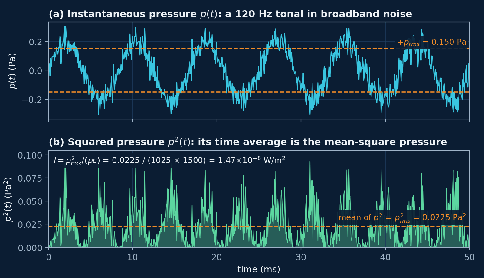
Because \( p(t) \) swings either side of zero, its plain average is close to zero and says nothing about how loud the sound is. Its size is measured by the mean-square pressure, the average of \( p^2 \) over a time \( T \),
and by its square root, the root-mean-square (RMS) pressure,
For \( N \) samples,
The RMS pressure, and its square, is the basis of SPL, band levels, the integral of the PSD and the detectability rule below.
Tonal, broadband, transient and ambient noise
The noise a vessel radiates into the water has three main components that matter for classifying vessels: tonal, broadband and transient. Their physical origins set their spectral structure, and that structure is what a classifier learns from (Urick 1983).
Tonal components
Tonals are narrow spectral lines from periodic mechanical motion: shaft rotation, gearbox meshing, electrical generators and their harmonics, and the propeller's blade rate. The blade-rate frequency, the rate at which the propeller's blades pass a fixed point, is
where \( B \) is the number of blades on the propeller and \( n_{\mathrm{shaft}} \) is the shaft speed in revolutions per minute (rpm). At a steady shaft speed these lines are stable, so they act as identifiers of the machinery that made them. The shaft speeds below are illustrative values inside the shaft-rate ranges the synthetic dataset uses for each vessel class:
Example 1 · blade-rate frequency
def blade_rate(blades, shaft_rpm):
    """Blade-rate frequency in Hz: f_BR = B * n_shaft / 60."""
    return blades * shaft_rpm / 60

for vessel, B, rpm in [("tanker", 3, 75), ("cargo ship", 4, 120),
                       ("fishing vessel", 5, 360), ("small craft", 3, 1200)]:
    f_br = blade_rate(B, rpm)
    print(f"{vessel:14s} B = {B}, {rpm:4d} rpm -> f_BR = {f_br:5.2f} Hz "
          f"(harmonics {2 * f_br:.2f}, {3 * f_br:.2f} Hz)")
Output
tanker         B = 3,   75 rpm -> f_BR =  3.75 Hz (harmonics 7.50, 11.25 Hz)
cargo ship     B = 4,  120 rpm -> f_BR =  8.00 Hz (harmonics 16.00, 24.00 Hz)
fishing vessel B = 5,  360 rpm -> f_BR = 30.00 Hz (harmonics 60.00, 90.00 Hz)
small craft    B = 3, 1200 rpm -> f_BR = 60.00 Hz (harmonics 120.00, 180.00 Hz)
The tanker and cargo-ship blade rates are a few hertz. The small craft's 60 Hz would sit off the conventional 0–50 Hz display of DEMON analysis (Detection of Envelope Modulation on Noise), a point the DEMON note takes up.
Broadband components
Broadband noise comes from hydrodynamic turbulence, flow noise, propeller cavitation (vapour bubbles forming and collapsing on the blades) and structural vibration. In a PSD it is a smooth spectrum without sharp peaks. It depends strongly on vessel speed.
Transient components
Transients are short events: the onset of cavitation, manoeuvring, mechanical impacts and other impulsive hydrodynamic events. They show as short bursts in the waveform and in a spectrogram (a display of the spectrum over successive short time windows).
Ambient noise
The ocean also has a persistent background, ambient noise, from wind and waves, distant shipping, marine life, rain and geophysical activity. Ambient-noise data are usually expressed as spectral density levels, in dB re 1 µPa²/Hz (Robinson et al. 2014, p. 52; the quantity is defined below), and Wenz (1962) is the classic survey of ambient-noise spectra and their sources. The synthetic-dataset note describes the sea-noise model used there.
Sound pressure level and the 1 µPa reference
The reference pressure, 1 µPa
A level in decibels (dB) is ten times the base-10 logarithm of the ratio of a power-like quantity, such as the mean-square pressure, to a reference value. Underwater acoustics uses the reference pressure
ISO 18405:2017, the international standard for underwater-acoustics terminology, gives 1 µPa as the reference value for sound pressure in underwater acoustics, and 1 µPa²/Hz for the mean-square sound pressure spectral density; the reference values are specified in ISO 1683:2015. Write the reference with every level, as in “dB re 1 µPa”: a level without its reference is not a measurement.
Why underwater and in-air decibels are not comparable
In air the reference sound pressure is 20 µPa; for sound in water and other media it is 1 µPa (IEC 60050-801, entry 801-22-07). The in-air value was chosen so that 0 dB corresponds to the threshold of hearing of a person with normal hearing at 1 kHz. The same pressure therefore reads \( 20\log_{10} 20 \approx 26 \) dB higher in water: a sound pressure labelled 0 dB in air would be labelled 26 dB in water (Chapman and Ellis 1998).
Two more differences make raw comparisons misleading. Water and air have widely different characteristic impedance \( \rho c \), density times sound speed: for seawater it is thousands of times the value for air, so equal pressures do not carry equal intensities (see acoustic intensity below). And a source level, referred to 1 m from the source, cannot be compared with a level received at some distance, a mix-up Chapman and Ellis (1998) found in published comparisons of sonar and jet-aircraft noise.
Sound pressure level (SPL)
Sound pressure level puts the RMS pressure on a decibel scale:
Because \( p_{\mathrm{rms}}^2 \) is proportional to acoustic intensity, \( 20\log_{10} \) of a pressure ratio is the same as \( 10\log_{10} \) of a power ratio: \( \mathrm{SPL} = 10\log_{10}\big(\overline{p^2}/p_{\mathrm{ref}}^2\big) \).
Example 2 · SPL from pressure samples
T = 5.0                     # clip length, s
N = int(fs * T)             # 80,000 samples
t = np.arange(N) / fs

# A 120 Hz machinery tonal (amplitude 0.2 Pa) in white noise (RMS 0.05 Pa)
p = 0.2 * np.sin(2 * np.pi * 120 * t) + 0.05 * rng.standard_normal(N)

p_rms = np.sqrt(np.mean(p**2))
spl = 20 * np.log10(p_rms / P_REF)
print(f"p_rms = {p_rms:.4f} Pa")
print(f"SPL   = {spl:.1f} dB re 1 µPa")
Output
p_rms = 0.1501 Pa
SPL   = 103.5 dB re 1 µPa
The tonal alone has an RMS pressure of \( 0.2/\sqrt{2} = 0.141 \) Pa and the noise 0.05 Pa. Their mean squares add, \( 0.0200 + 0.0025 = 0.0225 \) Pa², which gives 0.150 Pa and 103.5 dB re 1 µPa.
The +6 dB detectability rule
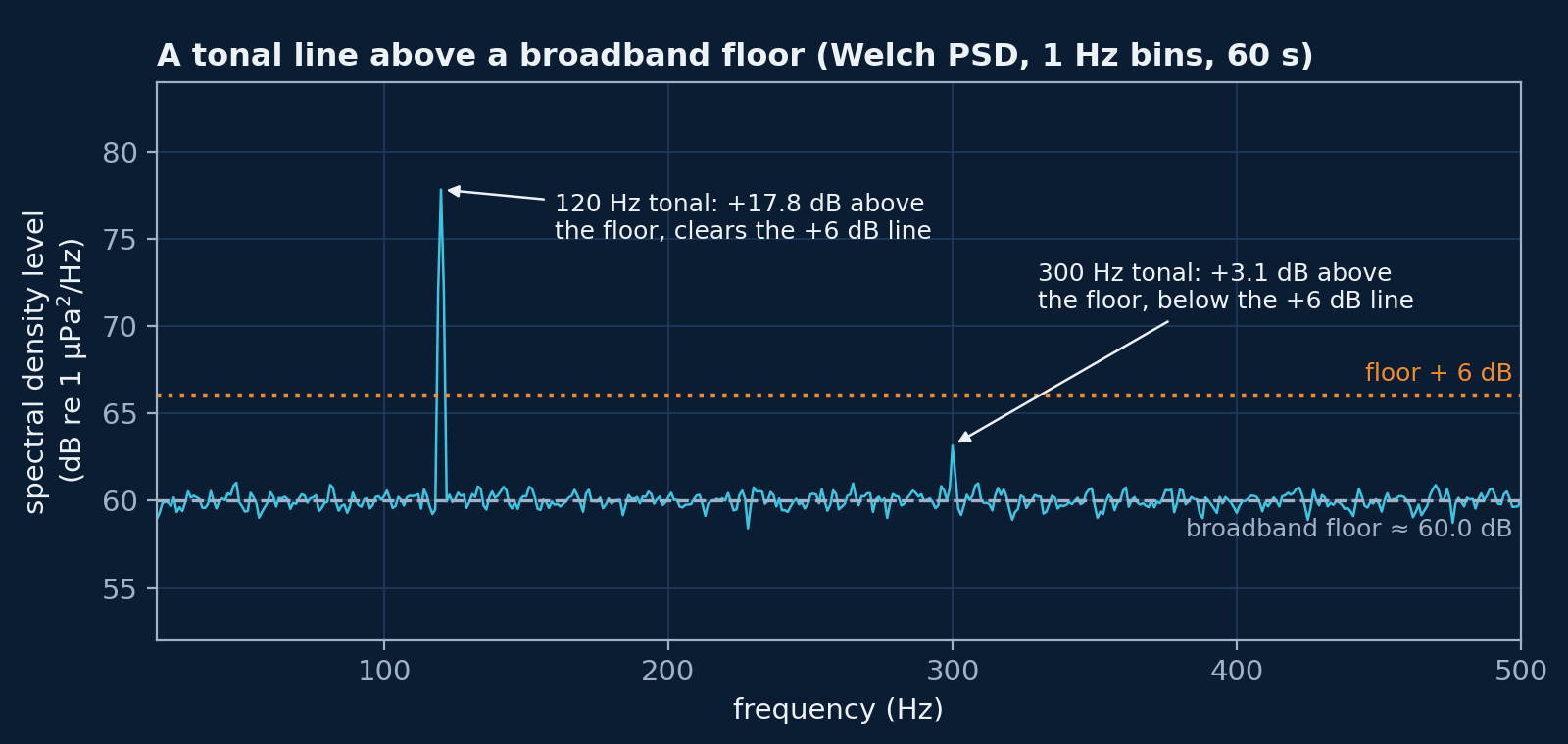
Detectability is expressed as a difference of levels in decibels, not as a raw ratio of powers. Let \( L_{\mathrm{sig}} \) be the signal level and \( L_{\mathrm{noise}} \) the noise level, both in dB and in the same band. The detectability threshold I use is
This corresponds to the signal's RMS pressure being about twice the ambient RMS pressure (a power ratio of about 4) in the same band. A +6 dB gap gives clear visibility of tonals and of many broadband features. The synthetic dataset mixes each vessel's noise at this gap above the sea noise, and Figure 2 shows the rule applied to tonal lines in a spectrum.
Spectra: the DFT, the PSD and band levels
The discrete Fourier transform and the FFT grid
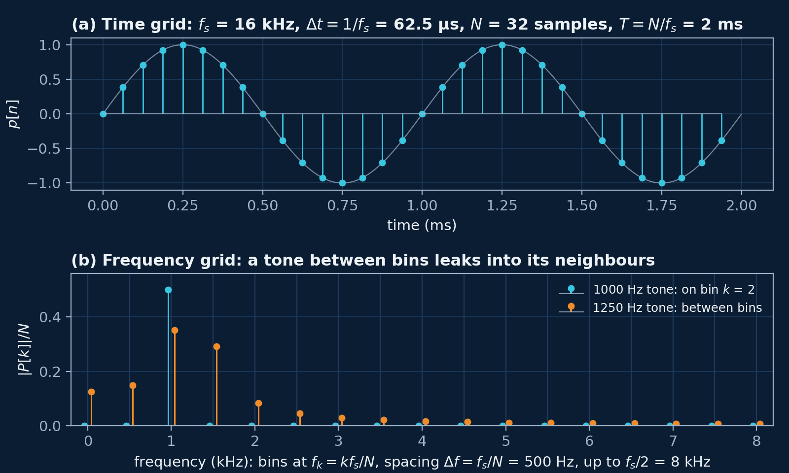
The discrete Fourier transform turns \( N \) samples into \( N \) complex coefficients, one per frequency bin:
The fast Fourier transform (FFT) is the standard fast algorithm for computing it. Bin \( k \) sits at
so the frequency resolution \( \Delta f \) is the inverse of the window length \( T = N/f_s \). For a real signal the bins that matter run from 0 Hz to the Nyquist frequency \( f_s/2 \), the highest frequency the sampled signal can represent; NumPy's rfft returns exactly those. At 16 kHz, a 1 s window (\( N \) = 16,000) gives 1 Hz bins up to 8 kHz.
The power spectral density (PSD)
The one-sided pressure PSD \( S_{pp}(f) \) is the mean-square pressure per unit bandwidth, in Pa²/Hz, over frequencies from 0 to \( f_s/2 \). A single-window estimate from the DFT, the periodogram (ignoring window effects), is
The factor 2 folds the negative frequencies onto the positive ones (the bins at 0 Hz and at \( f_s/2 \) are not doubled). A single periodogram is very noisy. Welch's method averages the periodograms of overlapping segments, each multiplied first by a window, a taper that reduces the leakage seen in Figure 1 (Welch 1967; Harris 1978). SciPy's welch with scaling="density" returns the one-sided PSD in Pa²/Hz:
Example 3 · Welch PSD with the right scaling
f, S = welch(p, fs=fs, window="hann", nperseg=fs, noverlap=fs // 2,
             scaling="density")            # one-sided PSD in Pa²/Hz, 1 Hz bins
df = f[1] - f[0]
print(f"Frequency resolution {df:.1f} Hz, {f.size} bins up to {f[-1]:.0f} Hz")
print(f"Mean-square pressure from the samples: {np.mean(p**2):.5f} Pa²")
print(f"Integral of the PSD (sum × Δf):        {np.sum(S) * df:.5f} Pa²")

level = 10 * np.log10(S / P_REF**2)        # dB re 1 µPa²/Hz
k = np.argmax(S)
print(f"Peak at {f[k]:.0f} Hz: {level[k]:.1f} dB re 1 µPa²/Hz")
print(f"Median level (the broadband floor): {np.median(level):.1f} dB re 1 µPa²/Hz")
Output
Frequency resolution 1.0 Hz, 8001 bins up to 8000 Hz
Mean-square pressure from the samples: 0.02254 Pa²
Integral of the PSD (sum × Δf):        0.02249 Pa²
Peak at 120 Hz: 101.3 dB re 1 µPa²/Hz
Median level (the broadband floor): 54.7 dB re 1 µPa²/Hz
The integral of the PSD matches the mean-square pressure of the samples, 0.02249 against 0.02254 Pa². This is Parseval's theorem (the mean square in time equals the integral of the PSD), and it is the check that a PSD's scaling is right. The broadband floor sits near 55 dB re 1 µPa²/Hz: the white noise's mean square, \( 0.05^2 = 0.0025 \) Pa², is spread evenly over 8 kHz, which is \( 3.1\times10^{-7} \) Pa²/Hz (Example 5 converts it to a level). The tonal stands about 47 dB above that floor in its bin.
A tonal puts all its power at one frequency, so its height in a PSD depends on the bin width and the window. Here the 120 Hz line's mean square, 0.02 Pa², is shared over the Hann window's equivalent noise bandwidth of 1.5 bins (Harris 1978), giving 0.0133 Pa²/Hz or 101.3 dB. A broadband floor does not change with the bin width. Quote tonals as band levels (next) to avoid this dependence.
Band level
The mean-square pressure in a band from \( f_1 \) to \( f_2 \) is the integral of the PSD over the band,
and the band level is
Note the unit: a band level is the level of a mean-square pressure, in dB re 1 µPa, not of a density.
Example 4 · band level from the PSD
def band_level(f, S, f1, f2):
    """Band level in dB re 1 µPa from a one-sided PSD in Pa²/Hz, over f1 <= f < f2."""
    m = (f >= f1) & (f < f2)
    ms = np.sum(S[m]) * (f[1] - f[0])      # mean-square pressure in the band, Pa²
    return 10 * np.log10(ms / P_REF**2)

L_broad = band_level(f, S, 1000, 2000)     # 1 kHz of broadband noise
floor = np.median(level[(f >= 1000) & (f < 2000)])
print(f"Band 1000-2000 Hz:                {L_broad:.1f} dB re 1 µPa")
print(f"PSD level + 10·log10(1000 Hz):    {floor + 10 * np.log10(1000):.1f} dB re 1 µPa")
L_tone = band_level(f, S, 110, 130)        # 20 Hz band around the tonal
print(f"Band 110-130 Hz (holds the tonal): {L_tone:.1f} dB re 1 µPa")
print(f"Tonal alone (0.2/√2 Pa RMS):       {20 * np.log10(0.2 / np.sqrt(2) / P_REF):.1f} dB re 1 µPa")
Output
Band 1000-2000 Hz:                84.8 dB re 1 µPa
PSD level + 10·log10(1000 Hz):    84.7 dB re 1 µPa
Band 110-130 Hz (holds the tonal): 103.0 dB re 1 µPa
Tonal alone (0.2/√2 Pa RMS):       103.0 dB re 1 µPa
For a flat PSD the band level is the PSD level plus \( 10\log_{10} \) of the bandwidth: 54.7 + 30 = 84.7 dB for a 1000 Hz band, against 84.8 dB from the integral. The 20 Hz band around the tonal gives 103.0 dB, the tonal's own level, whatever the bin width.
Noise level per hertz and the level in a 1 Hz band
Ambient-noise curves give the noise level as a spectral density level,
which converts back to a PSD as
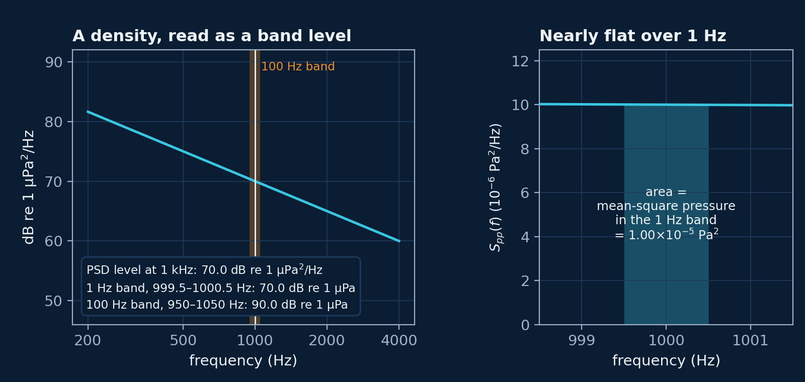
The mean-square pressure in a 1 Hz band centred on \( f_0 \) is
The two are related but are not the same quantity:
- \( S_{pp}(f) \) is a density, in Pa²/Hz, and \( \mathrm{NL}(f) \) is its level, in dB re 1 µPa²/Hz;
- integrating over 1 Hz gives the total mean-square pressure in that band, in Pa², and its level is in dB re 1 µPa.
When the PSD is roughly flat across the 1 Hz band, the integral is \( S_{pp}(f_0) \times 1\ \text{Hz} \), and the two levels are numerically equal: \( \mathrm{NL}(f_0) \) in dB re 1 µPa²/Hz is the level of the 1 Hz band in dB re 1 µPa. When the PSD changes within the band, as it does across a narrow tonal line, they differ. The synthetic dataset works with \( S_{pp}(f) \) as its primary spectral quantity throughout.
Example 5 · noise level (dB re 1 µPa²/Hz) <-> PSD (Pa²/Hz)
def nl_to_psd(nl_db):
    """Spectral density level in dB re 1 µPa²/Hz -> PSD in Pa²/Hz."""
    return P_REF**2 * 10 ** (np.asarray(nl_db) / 10)

def psd_to_nl(S_pa2_per_hz):
    """PSD in Pa²/Hz -> spectral density level in dB re 1 µPa²/Hz."""
    return 10 * np.log10(np.asarray(S_pa2_per_hz) / P_REF**2)

print(f"NL = 60 dB re 1 µPa²/Hz  ->  S = {nl_to_psd(60):.1e} Pa²/Hz")
print(f"S = 3.1e-07 Pa²/Hz       ->  NL = {psd_to_nl(3.1e-7):.1f} dB re 1 µPa²/Hz")
f0 = 1500
print(f"At {f0} Hz: NL = {level[f == f0][0]:.1f} dB re 1 µPa²/Hz; "
      f"level of the 1 Hz band = {band_level(f, S, f0 - 0.5, f0 + 0.5):.1f} dB re 1 µPa")
Output
NL = 60 dB re 1 µPa²/Hz  ->  S = 1.0e-06 Pa²/Hz
S = 3.1e-07 Pa²/Hz       ->  NL = 54.9 dB re 1 µPa²/Hz
At 1500 Hz: NL = 56.1 dB re 1 µPa²/Hz; level of the 1 Hz band = 56.1 dB re 1 µPa
With 1 Hz bins, the 1 Hz band at 1500 Hz is a single bin, so its level equals the PSD level there: 56.1 in both units. The white noise of Example 2, at \( 3.1\times10^{-7} \) Pa²/Hz, is 54.9 dB re 1 µPa²/Hz; the estimate at any one frequency scatters around that value.
Propagation and transmission loss
Spherical spreading
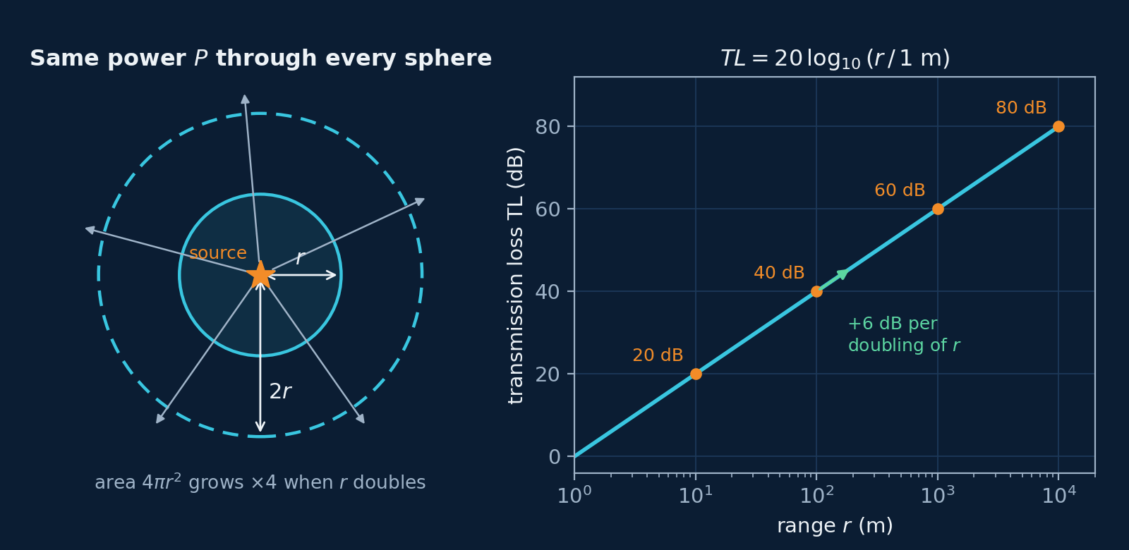
A point source radiating acoustic power \( P_{\mathrm{acoustic}} \), in watts, into a uniform, lossless medium spreads it over spheres of growing area, so the intensity at distance \( r \) is
For a plane wave, and for a spherical wave far enough from its source, intensity and RMS pressure are related by
where \( \rho \) is the water's density and \( c \) its sound speed. Together, these give
Transmission loss
Transmission loss is the reduction in level between two points in a sound field (ISO 18405:2017, 3.4.1.3). For spherical spreading, relative to a reference range \( r_0 \),
and with \( r_0 \) = 1 m, \( TL(r) = 20\log_{10} r \), with \( r \) in metres (Urick 1983). That is 6 dB per doubling of range, a property of spreading that has nothing to do with the +6 dB detectability rule. Spherical spreading is the simplest propagation model: it ignores absorption, reflection from the sea surface and seabed, and refraction, and it is the natural first model when range has to be simulated.
Source level and received level
Source level (SL) describes the source itself:
In practice it is a far-field quantity, measured where the pressure falls as \( 1/r \) and referred back to a nominal 1 m, not a pressure you would measure 1 m from a real ship (Robinson et al. 2014, p. 60). ISO 18405:2017 writes the reference value for source level as 1 µPa² m², and notes the widespread practice of quoting “dB re 1 µPa @ 1 m”; the numbers are the same. The received level (RL) at range \( r \) is
At \( r \) = 100 m, \( TL \approx 40 \) dB, so \( \mathrm{RL} \approx \mathrm{SL} - 40 \) dB.
Example 6 · spherical-spreading transmission loss
SL = 150.0                                  # illustrative source level, dB re 1 µPa at 1 m
for r in [1, 10, 100, 1_000, 10_000]:
    TL = 20 * np.log10(r / 1.0)             # r0 = 1 m
    RL = SL - TL
    print(f"r = {r:6d} m: TL = {TL:5.1f} dB, RL = {RL:5.1f} dB re 1 µPa, "
          f"p_rms = {P_REF * 10 ** (RL / 20):.2e} Pa")
Output
r =      1 m: TL =   0.0 dB, RL = 150.0 dB re 1 µPa, p_rms = 3.16e+01 Pa
r =     10 m: TL =  20.0 dB, RL = 130.0 dB re 1 µPa, p_rms = 3.16e+00 Pa
r =    100 m: TL =  40.0 dB, RL = 110.0 dB re 1 µPa, p_rms = 3.16e-01 Pa
r =   1000 m: TL =  60.0 dB, RL =  90.0 dB re 1 µPa, p_rms = 3.16e-02 Pa
r =  10000 m: TL =  80.0 dB, RL =  70.0 dB re 1 µPa, p_rms = 3.16e-03 Pa
Each factor of ten in range costs 20 dB and divides the RMS pressure by ten.
RMS pressure, p² and acoustic intensity
Mean-square pressure and RMS pressure, again
Because \( p(t) \) oscillates about zero, only the mean square \( \overline{p^2} \) carries the energy information.
Acoustic intensity
Acoustic intensity \( I \) is the acoustic power per unit area, in W/m². For a plane wave,
so intensity is proportional to \( p_{\mathrm{rms}}^2 \). The product \( \rho c \) is the medium's characteristic impedance; for seawater, with \( \rho \approx \) 1025 kg/m³ and \( c \approx \) 1500 m/s, it is about \( 1.54\times10^{6} \) Pa·s/m.
Synthesise p(t), not p²(t)
The tempting shortcut
Since levels depend on \( p^2 \), it is tempting to model \( p^2(t) \) directly. For synthesis, that is wrong:
- squaring creates new components at 0 Hz and at \( 2f_0 \) for every tone at \( f_0 \);
- squaring makes broadband Gaussian (normally distributed) noise non-Gaussian, and distorts its spectrum;
- the spectrum of \( p^2(t) \) is not the PSD of \( p(t) \), so as a description of the sound you want to make, \( \mathrm{FFT}[p^2(t)] \) has no physical meaning;
- the PSD of \( p(t) \) cannot in general be reconstructed from \( p^2(t) \).
Example 7 · what squaring does to a tone
x = np.sin(2 * np.pi * 120 * t)             # a pure 120 Hz tone
freqs = np.fft.rfftfreq(N, 1 / fs)
for name, sig in [("p(t)", x), ("p²(t)", x**2)]:
    spec = np.abs(np.fft.rfft(sig)) / N
    lines = freqs[spec > 0.01]
    print(f"{name:6s} spectral lines at: {', '.join(f'{v:.0f} Hz' for v in lines)}")
Output
p(t)   spectral lines at: 120 Hz
p²(t)  spectral lines at: 0 Hz, 240 Hz
A 120 Hz tone has one line; its square has lines at 0 Hz and 240 Hz, because \( \sin^2 x = (1 - \cos 2x)/2 \).
This is a statement about synthesis. Squaring, or taking the envelope, is a legitimate analysis step when the information is in the modulation: DEMON analysis demodulates cavitation noise and takes the spectrum of its envelope to read the blade rate (see the DEMON note). That is a different operation, asking a different question, and it does not make \( p^2(t) \) a model of the sound.
Synthesis from \( S_{pp}(f) \) to \( p(t) \)
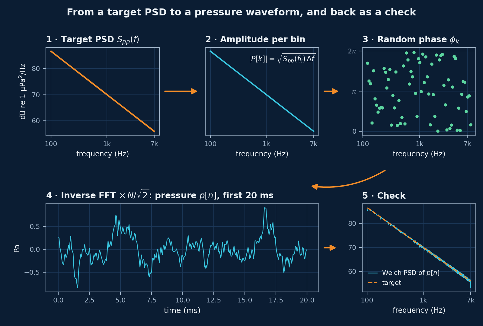
To make a pressure waveform with a chosen PSD:
- Choose \( f_s \), \( N \) and \( \Delta f = f_s/N \).
- Obtain the target PSD \( S_{pp}(f) \), in Pa²/Hz.
- Compute the amplitude spectrum: \( |P(f_k)| = \sqrt{S_{pp}(f_k)\,\Delta f} \).
- Assign random phases: \( \phi_k \sim \mathrm{Uniform}(0, 2\pi) \).
- Form the complex spectrum: \( P(f_k) = |P(f_k)|\,e^{j\phi_k} \).
- Impose Hermitian symmetry, \( P(-f_k) = P^*(f_k) \): each negative-frequency coefficient is the complex conjugate of its positive twin, which makes the time signal real. NumPy's
irfftdoes this for you. - Inverse FFT to get \( p[n] \). With NumPy's
irfft, multiply by \( N/\sqrt{2} \): \( N \) undoes the \( 1/N \) in NumPy's inverse transform, and \( 1/\sqrt{2} \) shares the one-sided PSD between positive and negative frequencies, so that the mean square of \( p[n] \) equals the integral of \( S_{pp} \). - Scale to the required RMS, if the clip must have a set level. With the factor in step 7, the RMS already matches the PSD.
Example 8 · synthesise p(t) from a target PSD
def synthesise(S_target, fs, N, rng):
    """Pressure waveform p[n] in Pa whose one-sided PSD is S_target(f) in Pa²/Hz."""
    freqs = np.fft.rfftfreq(N, 1 / fs)
    df = fs / N
    amp = np.sqrt(S_target(freqs) * df)            # |P[k]| = sqrt(S_pp(f_k) * Δf)
    amp[0] = 0.0                                   # no DC
    amp[-1] = 0.0                                  # leave the Nyquist bin empty
    phase = rng.uniform(0, 2 * np.pi, freqs.size)  # random phases
    # irfft imposes Hermitian symmetry (a real output) and divides by N; N/√2 restores
    # pascals, with the one-sided PSD shared between positive and negative frequencies
    return np.fft.irfft(amp * np.exp(1j * phase), n=N) * N / np.sqrt(2)

def target(freq):
    """70 dB re 1 µPa²/Hz at 1 kHz, falling 5 dB per octave, from 100 Hz to 7 kHz."""
    freq = np.asarray(freq, dtype=float)
    nl = 70 - 5 * np.log2(np.maximum(freq, 1.0) / 1000)
    return np.where((freq >= 100) & (freq <= 7000), nl_to_psd(nl), 0.0)

p_syn = synthesise(target, fs, N, rng)
f2, S2 = welch(p_syn, fs=fs, window="hann", nperseg=4096, scaling="density")
for fc in (250, 1000, 4000):
    band = (f2 >= 0.95 * fc) & (f2 <= 1.05 * fc)
    print(f"{fc:5d} Hz: target {psd_to_nl(target(fc)):.1f}, "
          f"synthesised {psd_to_nl(np.mean(S2[band])):.1f} dB re 1 µPa²/Hz")
expected = np.sqrt(np.sum(target(freqs)) * fs / N)
print(f"RMS of the synthesised p(t): {np.sqrt(np.mean(p_syn**2)):.3f} Pa (expected {expected:.3f} Pa)")
Output
  250 Hz: target 80.0, synthesised 80.1 dB re 1 µPa²/Hz
 1000 Hz: target 70.0, synthesised 69.9 dB re 1 µPa²/Hz
 4000 Hz: target 60.0, synthesised 60.0 dB re 1 µPa²/Hz
RMS of the synthesised p(t): 0.255 Pa (expected 0.255 Pa)
The synthesised waveform's PSD is within 0.1 dB of the target at 250 Hz, 1 kHz and 4 kHz, and its RMS equals the value the PSD predicts, 0.255 Pa.
In short
- Always synthesise pressure waveforms \( p(t) \).
- Use \( p^2(t) \) only for energy and level calculations.
- The PSD is the fundamental spectral quantity.
How this is used in SKANN
SKANN, the Selective-Kernel Acoustic Neural Network, is the deep-learning architecture for underwater audio that I developed at Oravont Systems; it takes the raw hydrophone waveform as its input. An earlier selective-kernel encoder, SKANN-SSL, was pretrained on my synthetic dataset with Barlow Twins, a self-supervised objective that makes the embeddings of paired clips agree while keeping their components decorrelated; its training pairs were drawn within each vessel class. The quantities on this page appear in that work as follows:
- \( p(t) \), in pascals, is the model input: SKANN reads the raw waveform, not a spectrogram.
- \( S_{pp}(f) \) is the input to sea-noise synthesis: the dataset's ambient noise is generated from a target PSD by the random-phase inverse-FFT method above, with the \( N/\sqrt{2} \) scaling, so the clips are in pascals.
- RMS pressure and SPL set the mix: each clip puts the vessel noise 6 dB above the sea noise, by RMS, following the +6 dB rule.
- Tonals and transients are why SKANN runs kernels of several lengths in parallel: no single analysis window resolves both slow machinery tonals and millisecond transients, so long kernels capture slow envelope structure and the tonal band, short kernels capture sharp transients, and selective-kernel attention learns which scales to trust for each input segment.
Symbols and units
| Symbol | Meaning | Unit |
|---|---|---|
| \( t \) | continuous time | s |
| \( n \) | sample index (integer) | – |
| \( f_s \) | sampling frequency | Hz |
| \( \Delta t \) | sampling interval, \( 1/f_s \) | s |
| \( N \) | number of samples per window | – |
| \( T \) | window duration, \( N/f_s \) | s |
| \( p(t) \) | instantaneous acoustic pressure | Pa |
| \( p[n] \) | discrete-time pressure sample | Pa |
| \( \overline{p^2} \) | mean-square acoustic pressure | Pa² |
| \( p_{\mathrm{rms}} \) | RMS acoustic pressure | Pa or µPa |
| \( p_{\mathrm{ref}} \) | reference pressure, 1 µPa | Pa |
| SPL | sound pressure level, \( 20\log_{10}(p_{\mathrm{rms}}/p_{\mathrm{ref}}) \) | dB re 1 µPa |
| \( \mathrm{NL}(f) \) | noise level (spectral density level) | dB re 1 µPa²/Hz |
| \( S_{pp}(f) \) | one-sided pressure PSD | Pa²/Hz |
| \( L_{[f_1,f_2]} \) | band level | dB re 1 µPa |
| SNR | signal-to-noise ratio, \( L_{\mathrm{sig}} - L_{\mathrm{noise}} \) | dB |
| \( r \) | range (distance from the source) | m |
| \( r_0 \) | reference range (usually 1 m) | m |
| TL | transmission loss | dB |
| SL | source level | dB re 1 µPa at 1 m (ISO 18405: dB re 1 µPa² m²) |
| RL | received level | dB re 1 µPa |
| \( \rho \) | density of seawater, about 1025 | kg/m³ |
| \( c \) | sound speed in seawater, about 1500 | m/s |
| \( I \) | acoustic intensity | W/m² |
| \( f \) | frequency | Hz |
| \( f_k \) | DFT bin frequency, \( k f_s/N \) | Hz |
| \( \Delta f \) | frequency resolution, \( f_s/N \) | Hz |
| \( P(f) \) | Fourier transform of \( p(t) \) | – |
| \( P[k] \) | DFT of \( p[n] \) | – |
| \( B \) | number of propeller blades | – |
| \( n_{\mathrm{shaft}} \) | shaft speed | rpm |
| \( f_{BR} \) | blade-rate frequency | Hz |
| \( \phi_k \) | random phase for bin \( k \), uniform in \( [0, 2\pi) \) | rad |
| IFFT | inverse discrete Fourier transform, computed by FFT | – |
Sources
- Chapman, D.M.F. and Ellis, D.D. (1998). The elusive decibel: thoughts on sonars and marine mammals. Canadian Acoustics 26(2), 29–31. jcaa.caa-aca.ca/index.php/jcaa/article/view/1125
- Harris, F.J. (1978). On the use of windows for harmonic analysis with the discrete Fourier transform. Proceedings of the IEEE 66(1), 51–83. doi:10.1109/PROC.1978.10837
- IEC 60050-801:1994. International Electrotechnical Vocabulary, Part 801: Acoustics and electroacoustics. Entry 801-22-07, sound pressure level. electropedia.org, 801-22-07
- ISO 1683:2015. Acoustics — Preferred reference values for acoustical and vibratory levels. iso.org/standard/64648.html
- ISO 18405:2017. Underwater acoustics — Terminology. iso.org/standard/62406.html
- Robinson, S.P., Lepper, P.A. and Hazelwood, R.A. (2014). Good Practice Guide for Underwater Noise Measurement. NPL Good Practice Guide No. 133, National Physical Laboratory. ISSN 1368-6550. eprintspublications.npl.co.uk/6121
- Urick, R.J. (1983). Principles of Underwater Sound, 3rd edn. McGraw-Hill. ISBN 0-07-066087-5.
- Welch, P.D. (1967). The use of fast Fourier transform for the estimation of power spectra: a method based on time averaging over short, modified periodograms. IEEE Transactions on Audio and Electroacoustics 15(2), 70–73. doi:10.1109/TAU.1967.1161901
- Wenz, G.M. (1962). Acoustic ambient noise in the ocean: spectra and sources. Journal of the Acoustical Society of America 34(12), 1936–1956. doi:10.1121/1.1909155
All figures on this page are generated from the formulas and signals above; none is taken from these sources.