← suniltyagi.in · Working notes

A Physics-Grounded Synthetic Underwater Acoustic Dataset
Full-factorial waveform generation from first-principle acoustic models, with corrected ambient noise, physics-based cavitation, and worked verification calculations
1. Introduction
Passive acoustic monitoring is a cornerstone of underwater domain awareness. Hydrophone arrays deployed on the seabed, towed behind ships, or integrated into autonomous buoys continuously record the acoustic environment. The challenge is not data collection — it is interpretation. Real underwater recordings are voluminous, unlabelled, and expensive to annotate. This creates a fundamental bottleneck for machine learning approaches that require labelled training data.
Classical sonar analysis — LOFAR (Low Frequency Analysis and Recording), DEMON (Detection of Envelope Modulation on Noise), and spectrogram interpretation — remains the standard for vessel classification. These methods are powerful but require trained operators and cannot scale to persistent, autonomous monitoring across wide maritime areas.
This article describes the design, physics, and verification of a synthetic underwater acoustic dataset built to address this gap. The dataset provides 12,000 physics-grounded waveforms covering four vessel classes and ambient ocean noise, generated from first-principle acoustic models with full-factorial parameter coverage. All quantities are maintained in physical units (Pascals, dB re 1 µPa) and verified against classical acoustic references.
When used to pre-train an encoder with the Barlow Twins self-supervised objective, with training pairs drawn within each class, this dataset produced embeddings with a silhouette score of 0.97 and 100% k-NN classification accuracy across five classes, measured on the same clips used for training.
2. System Architecture
The generation pipeline consists of two parallel synthesis branches — sea noise and ship noise — combined at a controlled signal-to-noise ratio.
Both branches output pressure waveforms in Pascals. The combined output is a 5-second clip at 16 kHz sampling rate (80,000 samples), stored as float32. All synthesis is constrained to the band 10 Hz – 8,000 Hz (Nyquist).
3. Acoustic Foundations
For a fuller treatment of these quantities, with runnable Python examples, see the tutorial Underwater acoustics for machine-learning engineers.
3.1 Reference Pressure and SPL
Underwater acoustics uses a reference pressure of:
Sound Pressure Level (SPL) is defined as:
where the RMS pressure over \( N \) discrete samples is:
3.2 Power Spectral Density vs 1 Hz Noise Level
The pressure PSD \( S_{pp}(f) \) is a density in Pa²/Hz; it is not the same quantity as a noise level. Ambient-noise curves such as Knudsen’s and Wenz’s give the noise level as a spectral density level; with the 1 µPa reference it is:
The level of the mean-square pressure in a 1 Hz band (dB re 1 µPa) equals \( \text{NL}(f) \) numerically when the PSD is roughly flat across that band; the units still differ. This dataset uses \( S_{pp}(f) \) as the primary spectral quantity throughout.
3.3 The +6 dB Detectability Rule
A +6 dB gap corresponds to the signal's RMS pressure being approximately twice the ambient level (power ratio of 4×), providing clear visibility of tonal lines and broadband features in standard LOFAR and DEMON analysis.
3.4 The \( p^2 \) vs \( p \) Synthesis Rule
Modelling \( p^2(t) \) directly is incorrect because squaring introduces spectral components at \( 2f \) for every tone at \( f \), distorts broadband Gaussian statistics, and makes PSD reconstruction impossible. The correct procedure is always:
\( \text{PSD} \) \( \;\rightarrow\; \text{amplitude spectrum} \) \( \;\rightarrow\; \text{random phase} \) \( \;\rightarrow\; \text{IFFT} \) \( \;\rightarrow\; p(t) \)
4. Sea Noise Model
Sea noise is generated using a piecewise parametric model based on digitised Knudsen curves.
4.1 Knudsen Model
The noise level (NL) in each frequency band follows:
where \( a \) (slope) and \( b \) (intercept) are fitted from digitised Knudsen curves for each sea state.
4.2 Frequency Bands
| Band | Frequency Range | Physical Mechanism | Behaviour |
|---|---|---|---|
| Turbulence | 10 Hz – \( f_t \) (~38 Hz) | Hydrodynamic turbulence | Flat plateau |
| LF | \( f_t \) – 200 Hz | Wind/ | Rising |
| MF | 200 Hz – 500 Hz | Transition | Mid-frequency shoulder, seen in the digitised Knudsen curves |
| HF | 500 Hz – 8,000 Hz | Wind-driven | Decay |
The turbulence–LF transition frequency \( f_t \) is calculated as the intersection of the turbulence plateau and the LF regression line:
Using SS3 fitted coefficients \( b_{\text{turb}} = 57.75 \), \( b_{\text{LF}} = 36.29 \), \( a_{\text{LF}} = 13.30 \):
\[ f_t = 10^{\,(57.75 - 36.29)/13.30} = 10^{1.614} = 41.1 \;\text{Hz} \]
This places the turbulence–wind transition in the expected range for moderate sea states.
4.3 Waveform Synthesis (IFFT Method)
The sea noise waveform is generated via spectral synthesis:
Step 1. Compute target PSD from Knudsen model:
\[ S_{pp}(f_k) = p_{\text{ref}}^2 \times 10^{\,\text{NL}(f_k)/10} \]Step 2. Convert PSD to amplitude spectrum:
\[ A[k] = \sqrt{S_{pp}(f_k) \cdot \Delta f} \quad \text{where } \Delta f = f_s / N \]Step 3. Apply random phases:
\[ \phi[k] \sim \mathcal{U}(0, 2\pi) \]Step 4. Construct complex spectrum:
\[ X[k] = A[k] \cdot e^{j\phi[k]}, \quad X[N-k] = X^*[k] \]Step 5. Inverse FFT with scaling:
\[ p[n] = \frac{N}{\sqrt{2}} \cdot \text{IFFT}\{X[k]\} \]The \( N/\sqrt{2} \) factor undoes the \( 1/N \) of the inverse FFT (as NumPy defines it) and shares the one-sided PSD between positive and negative frequencies, so that the waveform’s mean-square pressure equals the integral of \( S_{pp}(f) \) (Parseval’s theorem) and the output is in pascals. The generator applies it to NumPy’s irfft.
4.4 Sea State Levels
| Sea State | RMS (Pa) | SPL (dB re 1 µPa) | Description |
|---|---|---|---|
| 0 | 0.0076 | 77.6 | Calm (glassy) |
| 1 | 0.0219 | 86.8 | Light air |
| 3 | 0.0725 | 97.2 | Gentle breeze |
| 6 | 0.1518 | 103.6 | Strong breeze |
These are the levels of the published dataset: every clip of a sea state has the same sea-noise RMS (manifest columns sea_rms_pa and sea_spl_db).

5. Ship Noise Model
Ship noise is generated using a hybrid approach: spectral synthesis for deterministic components and a physical burst model for cavitation.
5.1 Vessel Classes
| Vessel Class | Shaft Rate (Hz) | Blades | BPF Range (Hz) | Cav. Peak (Hz) |
|---|---|---|---|---|
| Tanker | 1.0 – 1.5 | 3, 4, 5 | 3 – 7.5 | 400 |
| Cargo Ship | 1.5 – 2.5 | 3, 4, 5 | 4.5 – 12.5 | 600 |
| Fishing Vessel | 4.0 – 8.0 | 3, 4, 5 | 12 – 40 | 1,500 |
| Small Craft | 15.0 – 30.0 | 3, 4, 5 | 45 – 150 | 5,000 |
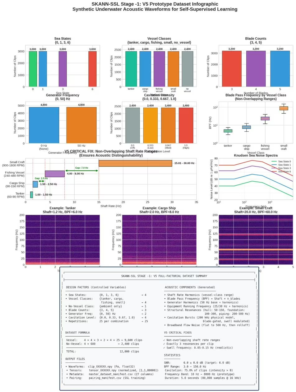
The shaft rate ranges are non-overlapping — a critical design decision. Earlier versions used overlapping ranges (fishing vessels 3–8 Hz, small craft 5–12 Hz), which caused catastrophic failure in downstream representation learning. The non-overlapping design ensures acoustic distinguishability at the fundamental tonal level.
5.2 Acoustic Components
The ship noise signal comprises six component types:
1. Shaft Rate Harmonics.
where \( f_0 \) is the shaft rotation frequency. Amplitude decays at 3 dB per harmonic.
2. Blade Pass Frequency (BPF) Harmonics.
BPF is the dominant tonal component. Amplitude decays at 4 dB per harmonic.
Cargo ship with \( f_0 = 2.0 \) Hz, \( n_{\text{blades}} = 4 \):
Shaft harmonics: 2.0, 4.0, 6.0, 8.0 Hz, …
BPF = \( 2.0 \times 4 = 8.0 \) Hz
BPF harmonics: 8.0, 16.0, 24.0, 32.0 Hz, …
All within the low-frequency band critical for long-range detection in LOFAR analysis.
3. Generator Harmonics.
Level is 10 dB below shaft harmonics.
4. Equipment Running Frequency. Shipboard machinery (pumps, compressors, fans) at synchronous motor speed: 25 Hz (50 Hz supply, 1500 RPM) or 30 Hz (60 Hz supply, 1800 RPM). Level is 15 dB below shaft harmonics with 4–7 harmonics.
5. Structural Resonances. Random narrowband tonals from ship structure: hull modes (50–150 Hz), foundation/mounting (100–300 Hz), piping/ductwork (200–500 Hz). Three resonances are selected per clip, 15 dB below shaft harmonics.
6. Broadband Flow Noise. Flow/turbulence noise with a frequency-dependent spectrum:
Flat below 500 Hz, then −3 dB/octave rolloff.
5.3 Cavitation Burst Model
Cavitation is modelled as discrete bubble collapse events using a physical approach.
Generation at 200 kHz. Bursts are generated at 200 kHz sampling rate (5 µs resolution) to capture the microsecond-scale collapse physics, then downsampled to 16 kHz with anti-aliasing.
Blade-gated timing. Bursts occur within activity windows synchronised to blade passage:
where \( T_{\text{blade}} = 1/f_{\text{BPF}} \) and \( I_{\text{cav}} \in [0, 1] \) is cavitation intensity.
Burst types. Three burst envelope types with different physical origins:
| Type | Proportion | Envelope | Duration |
|---|---|---|---|
| Collapse | 60% | Sharp attack, exponential decay | 10 – 100 µs |
| Cloud | 30% | Gaussian envelope | 100 µs – 1 ms |
| Sheet | 10% | Oscillatory | 1 – 10 ms |
Rayleigh collapse time. The single-bubble collapse duration is:
where \( R_{\text{bubble}} \sim \text{LogNormal}(\ln(50\;\mu\text{m}),\; 0.5) \).
For a bubble with \( R = 50 \; \mu\text{m} = 5 \times 10^{-5} \; \text{m} \), \( \rho = 1025 \; \text{kg/m}^3 \), \( \Delta P = 10^5 \; \text{Pa} \) (1 atm):
\[ \tau = 0.915 \times 5 \times 10^{-5} \times \sqrt{\frac{1025}{10^5}} = 4.575 \times 10^{-5} \times \sqrt{0.01025} \]
\[ = 4.575 \times 10^{-5} \times 0.1012 = 4.63 \;\mu\text{s} \]
At 200 kHz (\( T_s = 5 \;\mu\text{s} \)), this collapse occupies approximately 1 sample — confirming why 200 kHz generation is necessary. Larger bubbles (100–500 µm) produce collapses of 10–100 µs, requiring 2–20 samples at 200 kHz.
Chaos parameters. Three randomisation factors create realistic spectrograms: intensity variation (±20% per blade, simulating wake non-uniformity), RPM jitter (±2% timing noise from governor hunting), and envelope wander (0.5 Hz modulation from sea state effects).
Raw burst amplitude is scaled by a gain factor (CAVITATION_GAIN = 0.001) to achieve approximately −10 dB relative to tonal components.
6. SNR-Controlled Mixing
The ship and sea waveforms are combined at a controlled signal-to-noise ratio:
The ship waveform is scaled by:
\[ \text{scale} = \frac{\text{RMS}_{\text{sea}} \times 10^{6/20}}{\text{RMS}_{\text{ship,raw}}} \]Combined waveform:
\[ x_{\text{combined}}(t) = x_{\text{sea}}(t) + \text{scale} \cdot x_{\text{ship,raw}}(t) \]7. Physical Units Verification
All output levels were verified against classical acoustic references. The following worked example uses Sea State 3 as the reference condition.
Sea noise:
\[ p_{\text{rms,sea}} = 0.0725 \;\text{Pa} \]
\[ \text{SPL}_{\text{sea}} = 20 \log_{10}\!\left(\frac{0.0725}{10^{-6}}\right) = 20 \times 4.860 = 97.2 \;\text{dB re } 1\;\mu\text{Pa} \quad \checkmark \]
Ship noise at +6 dB:
\[ p_{\text{rms,ship}} = 0.0725 \times 10^{6/20} = 0.0725 \times 1.9953 = 0.1447 \;\text{Pa} \]
\[ \text{SPL}_{\text{ship}} = 20 \log_{10}\!\left(\frac{0.1447}{10^{-6}}\right) = 103.2 \;\text{dB re } 1\;\mu\text{Pa} \quad \checkmark \]
Combined signal (power addition):
\[ p_{\text{rms,combined}} = \sqrt{p_{\text{rms,sea}}^2 + p_{\text{rms,ship}}^2} = \sqrt{0.0725^2 + 0.1447^2} \]
\[ = \sqrt{0.005256 + 0.020926} = \sqrt{0.026182} = 0.1618 \;\text{Pa} \]
\[ \text{SPL}_{\text{combined}} = 20 \log_{10}\!\left(\frac{0.1618}{10^{-6}}\right) = 104.2 \;\text{dB re } 1\;\mu\text{Pa} \quad \checkmark \]
Verification: combined SPL (104.2 dB) is 1.0 dB above ship SPL (103.2 dB), which is the expected result for incoherent addition of two signals where one is 6 dB below the other. The manifest gives 103.2 dB and 104.1–104.2 dB for the ship and combined levels of every sea-state-3 vessel clip. ✓
8. Full-Factorial Dataset Design
8.1 Design Factors
| Factor | Levels | Count | Notes |
|---|---|---|---|
| Sea State | {0, 1, 3, 6} | 4 | Knudsen model |
| Vessel Class | {small_craft, fishing, cargo, tanker} | 4 | Determines shaft rate range |
| Blade Count | {3, 4, 5} | 3 | Overrides vessel default |
| Generator Freq | {0, 50} Hz | 2 | 0 = no generator |
| Cav. Intensity | {0.0, 0.333, 0.667, 1.0} | 4 | 0.0 = no cavitation |
8.2 Dataset Size
8.3 Randomised Parameters
Within each factorial combination, the following are randomised per repetition: shaft rate (within vessel class range), structural resonance frequencies (three per clip), cavitation burst timing and carrier frequencies, phase of all spectral components, and the sea noise realisation.
8.4 Reproducibility
Separate RNG streams for sea noise (seed + 1) and ship noise (seed + 2) ensure bitwise reproducibility.
9. Spectral Analysis Validation
To verify that the generator produces acoustically realistic waveforms, individual clips were analysed using the same classical sonar techniques applied to real hydrophone recordings. The following example uses a cargo ship clip with 4 blades, shaft rate 2 Hz (120 RPM), BPF = 8 Hz, equipment at 25 Hz (1500 RPM), and cavitation at 759 Hz and 3200 Hz.
9.1 LOFAR Display (0–30 Hz)
The LOFAR (Low Frequency Analysis and Recording) display shows the narrowband tonal structure in the low-frequency regime. All expected spectral lines are present at their correct frequencies:

Figure 1: LOFAR Display (0–30 Hz) — Shaft frequency at 2 Hz, 2×Shaft at 4 Hz, BPF at 8 Hz with 2×BPF harmonic at 16 Hz, and Equipment running frequency at 25 Hz. All lines are stable across the 1-second observation window, consistent with steady-state vessel transit.
The shaft rate (2 Hz) and its second harmonic (4 Hz) are clearly visible. The blade-pass frequency at 8 Hz is the dominant tonal, with its second harmonic at 16 Hz. The equipment line at 25 Hz (corresponding to a 50 Hz supply, 1500 RPM synchronous motor) appears at the expected position. This tonal ladder is exactly what a sonar operator would see on a real LOFAR gram of a cargo vessel.
9.2 Wideband Spectrogram (0–8 kHz)
The wideband spectrogram reveals the mid- and high-frequency structure, including cavitation bands and generator harmonics:

Figure 2: Spectrogram (0–8 kHz) — Cavitation energy concentrated at 759 Hz and 3200 Hz (blade-gated bursts), with 50 Hz generator harmonics visible in the low-frequency band. The broadband flow noise floor shows the expected −3 dB/octave rolloff above 500 Hz.
The two cavitation bands are clearly separated, matching the generator's vessel-specific peak frequencies. The 50 Hz generator harmonics form a regular comb pattern in the lowest portion of the spectrogram. The ambient noise floor follows the expected spectral shape from the corrected Knudsen model.
9.3 DEMON Analysis
DEMON (Detection of Envelope Modulation on Noise) analysis extracts the modulation spectrum from the cavitation band (759–3200 Hz). This technique reveals the shaft rate and blade-pass modulation imposed on the broadband cavitation noise:

Figure 3: DEMON Analysis (cavitation band 759–3200 Hz) — Clear modulation peaks at shaft rate (2 Hz), BPF (8 Hz), and BPF harmonics (16, 24, 32, 40 Hz). The 3×shaft sideband structure (6 Hz) is also visible, confirming blade-gated cavitation timing.
The DEMON output confirms that the cavitation burst model's blade-gated timing produces the correct modulation structure. The dominant peak at 8 Hz (BPF) with harmonics at 16, 24, 32, and 40 Hz is precisely what DEMON analysis extracts from real cavitating vessels. The shaft rate (2 Hz) and its harmonics appear as sidebands, confirming that the burst timing is properly synchronised to propeller rotation.
These three independent analyses — LOFAR, spectrogram, and DEMON — validate that the synthetic waveforms contain the acoustic signatures that classical sonar techniques are designed to detect, at the correct frequencies and with realistic spectral relationships.
10. Downstream Validation
The dataset was used to pre-train an encoder with the Barlow Twins self-supervised objective (512-dim backbone embeddings). The pairing manifest defined positive pairs by shared vessel class, so class labels guided which clips were paired; there was no classification loss.
| Metric | Value |
|---|---|
| Silhouette Score (cosine, backbone, training clips) | 0.9697 |
| k-NN Accuracy (k=5, 5-fold CV, training clips) | 100% |
| Class labels | Used to choose training pairs (within each class); no classification loss |
| Classes | 5 (tanker, cargo, fishing, small craft, ambient) |
The silhouette score of 0.97 indicates near-perfect cluster separation of the training clips: the physics-grounded synthetic data carries enough acoustic structure for an encoder trained on within-class pairs to learn discriminative vessel representations. The k-NN folds split the embeddings, but the encoder had already been trained on all 12,000 clips, so neither figure is a test on unseen clips or real recordings.
11. Known Limitations
1. Doppler not implemented. Doppler-induced frequency shifts from relative vessel–hydrophone motion were deprioritised. Can be added as post-processing if needed for CPA (Closest Point of Approach) scenarios.
2. Single-source model. Each clip contains one vessel (or ambient only). Multi-source scenarios — multiple simultaneous vessels at different bearings and ranges — require extension of the mixing pipeline.
3. Stationary statistics. Each clip has fixed acoustic parameters throughout its 5-second duration. Time-varying scenarios such as CPA approach geometry, speed changes, or manoeuvring events are not modelled.
4. No propagation effects. Multipath arrivals, surface and bottom reflections, range-dependent attenuation, and shallow-water waveguide effects are not included. The current model assumes a direct-path, range-independent scenario.
5. Synthetic only. The dataset has not yet been validated against labelled real-world recordings. Integration with publicly available datasets (NOAA NCEI Passive Acoustic Archives, MBARI Hydrophone Dataset, JAMSTEC Underwater Observatory Recordings, DCLDE Workshop Datasets) is planned for final validation.
12. Dataset Availability
The full dataset is publicly available under CC BY 4.0:
Hugging Face: huggingface.co/datasets/suniltyagi/underwater-acoustic-synthetic-dataset · DOI 10.57967/hf/11191
Source repository: github.com/suniltyagialtair/Underwater-Acoustic-Synthetic-Dataset
12,000 clips · 5 seconds each · 16 kHz · 4 vessel classes + ambient · Full-factorial design · All physical units in Pascals
Built by Oravont Systems LLP.
References
[1] Knudsen, V. O., Alford, R. S., Emling, J. W. (1948). "Underwater Ambient Noise." J. Marine Research, 7(3), 410–429.
[2] Wenz, G. M. (1962). "Acoustic Ambient Noise in the Ocean: Spectra and Sources." JASA, 34(12), 1936–1956.
[3] Ross, D. (1976). Mechanics of Underwater Noise. Pergamon Press.
[4] Urick, R. J. (1983). Principles of Underwater Sound. 3rd ed., McGraw-Hill.
[5] Rayleigh, Lord (1917). "On the Pressure Developed in a Liquid During the Collapse of a Spherical Cavity." Phil. Mag., 34, 94–98.
[6] Zbontar, J., Jing, L., Misra, I., LeCun, Y., Deny, S. (2021). "Barlow Twins: Self-Supervised Learning via Redundancy Reduction." ICML 2021.
About: This dataset was created by Sunil Tyagi (Oravont Systems LLP) for pretraining SKANN-SSL, a separate detection-and-classification model. SKANN for vessel re-identification is another separate encoder, described in arXiv:2609.07399.
Also published on LinkedIn · More working notes at suniltyagi.in