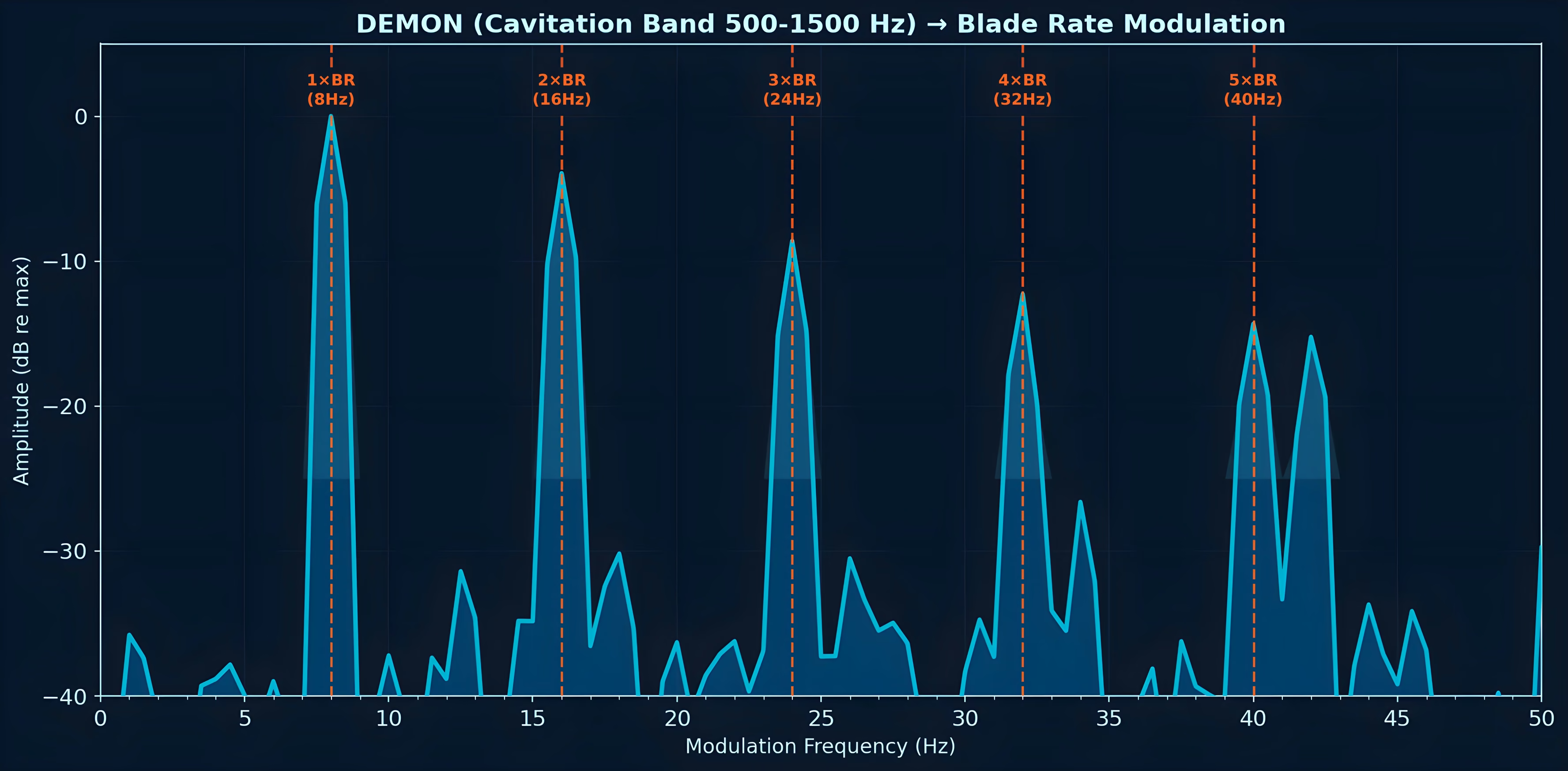
Why write this
Most of my current work applies deep learning to underwater acoustics — embeddings, metric learning, vessel re-identification. Yet one of the most useful tools on my bench is a signal-processing method from the analogue sonar era: DEMON — Detection of Envelope Modulation on Noise.
This note is a short, practical walk-through: what DEMON extracts, the four-step pipeline, how to read the output, the band-selection decision that most tutorials skip, and a case study where DEMON found a defect in a synthetic dataset that conventional spectrograms had hidden.
Everything here is textbook-level physics applied to open material. That is deliberate: the value of DEMON is precisely that it is transparent.
The physics in one paragraph
A cavitating propeller is a broadband noise source — collapsing vapour bubbles radiate across hundreds to thousands of hertz. But the cavitation is not steady. Each blade loads and unloads as it sweeps through the wake, so the broadband noise is amplitude-modulated at the blade-passage rhythm. The broadband cavitation is the carrier; the propeller kinematics are the modulation. DEMON demodulates the carrier and reads the rhythm.
Two relationships turn that rhythm into engineering numbers:
- Shaft rate: SR (Hz) = RPM / 60
- Blade rate: BR (Hz) = SR × number of blades
A shaft turning at 120 RPM drives SR = 2 Hz; with a four-bladed propeller, BR = 8 Hz. Recover SR and BR from a recording and you have inferred the propulsion configuration of a vessel you have never seen — from noise alone.
The pipeline, in four steps
- Bandpass the recording in a cavitation-dominated band. A common starting point is 500–2000 Hz, but this is vessel-dependent — more on that below.
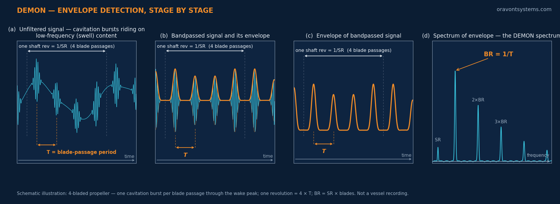
- Hilbert envelope. Take the analytic signal and extract its magnitude. This recovers the amplitude envelope — the modulation riding on the carrier.
- AC-couple the envelope. Remove the DC component and slow drift, so the spectrum is not dominated by a zero-frequency spike.
- FFT of the envelope. The result is a low-frequency modulation spectrum, typically displayed 0–50 Hz. This — not the spectrum of the raw signal — is the DEMON spectrum.
The conceptual point that makes DEMON click for newcomers: you are taking the spectrum of the envelope, not of the signal. The information lives in how the loudness fluctuates, not in the frequencies of the noise itself.
The maths in one paragraph
Envelope extraction rests on the Hilbert transform — an integral transform equivalent to convolving the signal with 1/(πt). Physically it is a special linear filter: every spectral component keeps its amplitude, but its phase is shifted by −π/2. Pairing the signal with this quadrature version of itself gives the analytic signal, and the envelope we are after is simply the analytic signal’s instantaneous magnitude. The three defining relations are set out below.
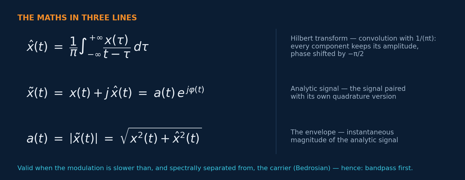
The magnitude recovers the amplitude modulation faithfully on one condition: the modulation must be spectrally separated from — and slower than — the carrier (Bedrosian’s theorem, in essence). That condition is the reason the pipeline is ordered the way it is. Bandpassing first isolates a carrier band in the hundreds-to-thousands of hertz, far above the few-hertz propulsion rhythms we want to read, so the two separate cleanly and the envelope means what we think it means. Skip the bandpass and low-frequency signal energy leaks into the “envelope” — you demodulate a mixture and read a comb that isn’t there, or miss one that is.
Reading the plot
A good DEMON spectrum of a cavitating vessel shows a harmonic comb: a line at the shaft rate, a stronger family at the blade rate and its integer multiples. The reading discipline is:
- Identify the fundamental of the dominant comb → candidate BR.
- Look for a weaker line at BR/N for small integer N → candidate SR, and N is the blade count.
- Check that BR harmonics (2×, 3×, 4× BR) line up. A comb that doesn’t repeat at integer multiples is telling you something else is modulating the band.
That last habit matters — it is what makes the case study below work.
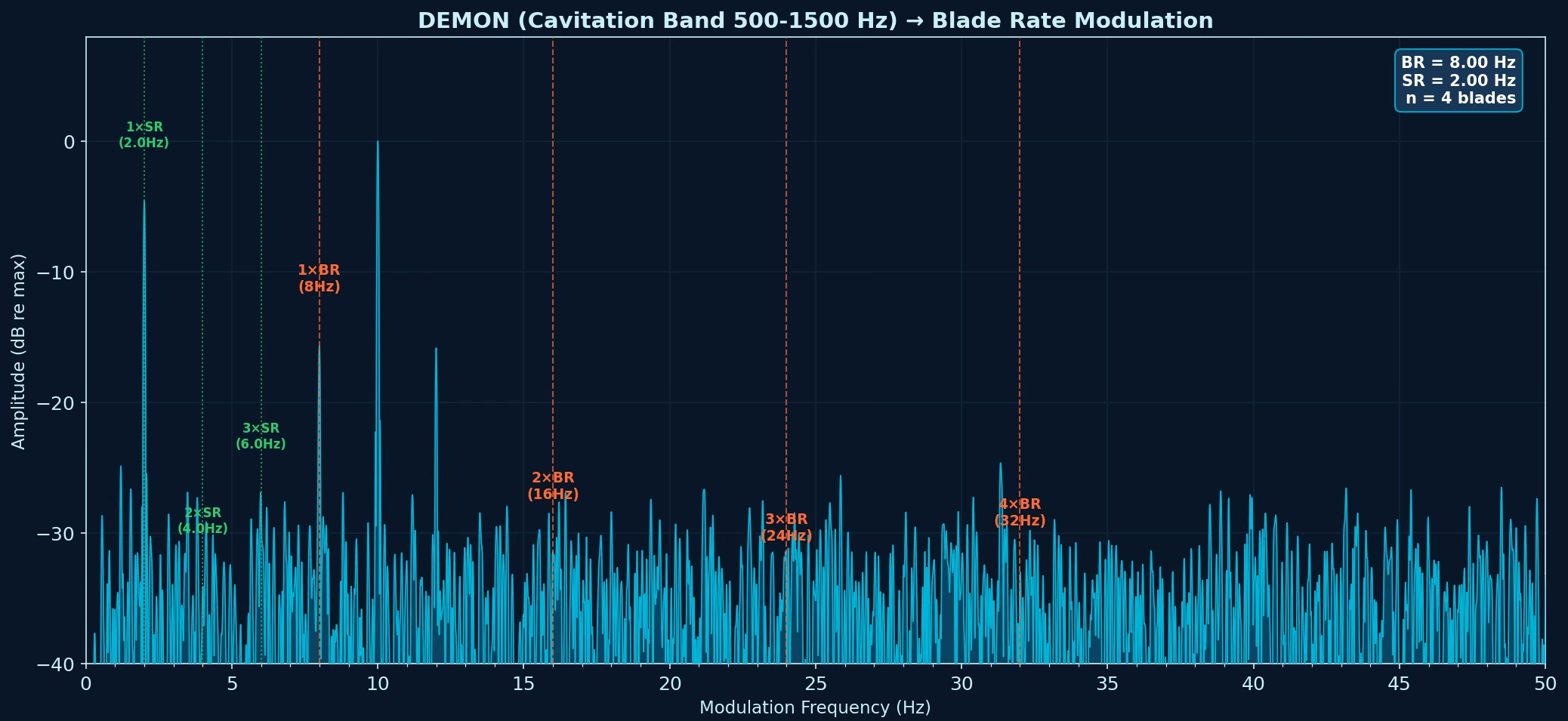
Figure 2 is worth a moment of honesty, because it shows why the reading discipline above is a discipline and not a formality. The tallest single line in this spectrum is not the blade rate — it sits at 10 Hz, a shaft-rate harmonic. Naive peak-picking would report the wrong fundamental. Comb reasoning gets it right: the family of lines spaced 2 Hz apart identifies SR = 2 Hz; the reinforced members of that family at 8, 16, 24, 32 Hz identify BR = 8 Hz; and BR/SR = 4 gives the blade count. Individual peak heights vary with propagation and band choice — the spacing of the comb is the robust observable.
The decision tutorials skip: which band, which display
Two defaults quietly shape every DEMON result: the bandpass band and the display range. Both are class-dependent, and getting them wrong produces a clean-looking plot of the wrong thing.
The band. Cavitation energy concentrates in different regions for different vessel types — a slow-turning tanker’s cavitation sits far lower in frequency than a fast small craft’s. Bandpass in a region the vessel doesn’t cavitate in, and you demodulate ambient noise.
The display. The conventional 0–50 Hz DEMON window is built around merchant-vessel assumptions. A fast small craft with a high shaft rate and several blades can put its blade rate well above 100 Hz — entirely off a 0–50 Hz plot. In validation runs on my synthetic dataset, the standard display missed the blade rate for the overwhelming majority of the small-craft class. The comb was there; the window wasn’t.
In practice there are two operating modes. If vessel class is known (or hypothesised), use class-specific bands and display ranges — this is ceiling performance. If it is not, the band itself becomes a search problem; I have had reasonable results letting a particle-swarm optimiser find the band that maximises comb structure, at the cost of compute and occasional convergence to the wrong region for atypical classes. The gap between the two modes is itself informative: it tells you how much a lightweight classifier front-end would buy you.
Case study: the swell artefact
The most useful thing DEMON has done for me recently had nothing to do with detecting a real vessel. I maintain a physics-grounded synthetic underwater acoustic dataset (openly released, CC BY 4.0) used for self-supervised pretraining. An earlier version of the generator produced clips that looked entirely plausible in spectrograms — the broadband structure, tonals and levels all passed visual inspection.
Run through DEMON, the clips told a different story. The generator applied sea-swell amplitude modulation at a fixed 0.5 Hz — and a fixed periodic modulation does not stay politely at its fundamental. Its harmonics printed lines at 1.0, 1.5, 2.0 Hz and beyond, leaking straight up into the 1–10 Hz band where shaft rates live. The worst of it: 2.0 Hz is a perfectly plausible shaft rate (120 RPM). An artefact that lands on top of a credible propulsion line is far more dangerous than an obviously spurious one — it can masquerade as a shaft-rate detection, or mask a genuine one.
Real ocean swell does not behave like this. It modulates received level at roughly 0.05–0.15 Hz — a 7–20 second period — well below the shaft-rate search band, gently, and with natural variability. The fix followed directly: randomise the swell frequency across that realistic range and keep the modulation depth modest, so swell remains the slow, gentle amplitude variation it is at sea. A regression check now flags any residual low-frequency comb on every dataset build.
Two lessons worth generalising:
- Synthetic data should be validated in the domain where it will be used. The artefact was invisible in the time-frequency views used to design the generator, and glaring in the modulation domain the downstream models actually learn from.
- A transparent physics tool is a superb QA instrument for ML pipelines. A neural network trained on those clips would happily have learned the swell harmonics as a “feature” — or learned to read a 2 Hz line that means nothing. DEMON, being nothing but physics, cannot be fooled into agreeing with your generator.
Where this sits in an AI-UDA workflow
I do not use DEMON instead of learned representations; I use it around them:
- Validation of synthetic and real clips before they enter training (as above).
- Interpretability: when an embedding model separates two recordings, DEMON often shows the physical reason — different blade rates, different comb structure — in a form a review board can read.
- Physics-grounded features: SR, BR and blade count are compact, meaningful descriptors that complement high-dimensional embeddings.
Classical DSP and deep learning are frequently framed as rivals. On the bench, the relationship is closer to auditor and analyst: the network finds structure at scale; the physics tells you whether to believe it.